FEA BOUNDARY CONDITIONS:
A PRACTICAL GUIDE FOR MECHANICAL ENGINEERS

FEA Boundary Conditions: A Practical Guide for Mechanical Engineers

Regardless of which finite element analysis (FEA) package you use, boundary conditions are among the most important modeling fundamentals to get right—and one of the most common sources of error. It’s tempting to quickly apply fixed constraints, run the model, and enjoy those beautiful stress contours. But, if you need your results to be more than pretty colors, you must think carefully about boundary conditions.

What Are Boundary Conditions?

In simple terms, boundary conditions are the conditions you impose on the boundaries of your model—your loads and constraints (and sometimes initial conditions). They define the question you’re asking with the analysis.

You may think you want a peak von Mises stress, but peak stress under which conditions?

Real boundary conditions are messy. Friction, contact, acceleration, thermal loading, complex load paths, bolted joints with preload, and fixture compliance can all matter. Modeling all of this is usually computationally expensive, impractical, and unnecessary. Like most engineering problems, the key is choosing simplified assumptions that fit your purpose.

The goal isn’t to avoid assumptions; assumptions and simplifications are necessary. The goal is to understand them, document them, and know when they’re appropriate.

A Practical Workflow: From Question to Constraints

Start with the question you want the model to answer.

Common questions include:

• • strength/yielding
  • deflection/stiffness
  • fatigue/durability
  • buckling
  • or modal/vibration response

That answer frames your approach and influences other modeling choices (for example; element type, material model, and whether contact is required). As you build the model, revisit that original question and ask whether each assumption could change the outcome you care about.

Next, develop a clear understanding of the loading and how it is reacted. If you don’t immediately have a mental picture of it, draw a free-body diagram (FBD). Even if you do have a mental picture, draw it anyway.

_{Even a very simple FBD will serve well when developing boundary conditions}.

Once you have a balanced free-body diagram, you’re most of the way to defining boundary conditions. The remaining catch is that we often simplify by neglecting gravity, friction, or secondary contacts (at least initially).  In the real world, these effects prevent parts from “floating” or sliding freely. If you neglect these stabilizing effects in an FEA model, the solver will still allow rigid-body motion unless you prevent it with constraints. The model must be fully constrained from rigid body motion to solve.  Normally this will become apparent in a couple of ways:

• In a linear static run, you’ll typically see solver warnings/errors such as singularities or excessive pivot ratios.
• In a nonlinear, multi-step run, the model may “walk away” or drift dramatically because rigid-body modes are not sufficiently restrained.

Even if your loading is “2D,” you still need to prevent rigid-body motion in the third dimension for the equations to be solvable. Often, these extra stabilizing constraints are where trouble starts - too few and the model won’t run; too many and you may introduce artificial stiffness and unintended load paths. The goal is to use stabilizing constraints that carry as little load as possible while still preventing rigid-body motion.

DOF and Element Behavior

Degrees of freedom (DOF) are the directions a node can move (and possibly rotate). Different element types have different DOFs:

• Solid elements: 3 translational DOF (Tx, Ty, Tz)
• Shell elements: 3 translations + 3 rotations (including a drilling rotation about the shell normal, depending on formulation)
• Beam elements: 3 translations + 3 rotations (6 total)

_{Nodal degrees of freedom (DOF) for 1D beams, 2D shell, and 3D solid elements.} 

A key implication: you cannot directly constrain rotational DOF on a solid element node—because that DOF doesn’t exist. Rotation is prevented indirectly by constraining translations at multiple nodes (creating a couple).

Common Boundary Condition Tools

Single-point constraints (SPCs)

SPCs are the most common constraint type—so common that many FEA tools simply label them “constraints.” SPCs can fix any available DOF at a node (or at nodes associated with a face/edge/geometry selection). Even when a tool lets you apply constraints to geometry or faces, the solver ultimately applies them at nodes.

Use “fixed” constraints only when the real boundary is truly rigid or when that rigidity assumption will not meaningfully affect the result you care about. Overuse of fixed constraints is a frequent source of overly stiff models and misleading stresses near the constraint. 

_{Using fixed constraints on the inside of these bolt holes (yellow regions) may get the model running quickly, but it will also add unnecessary stiffness to your model. Although this assumption is still more useful than fixing the entire bottom surface.}

Multi-Point Constraints (MPCs): RBE2 vs RBE3

MPCs are multi-point constraint equations that relate the motion of one node to one or more other nodes. In practice, this often refers to RBE2 and RBE3 elements, commonly visualized as “rigid spiders” when connecting a central node to a ring or surface of nodes.

RBEs are useful for:

• • Applying remote loads or boundary conditions to a region. 
  • Representing rigid fixtures or rigid parts (where appropriate).
  • Connecting elements with different DOFs (e.g., an idealized bolt modeled as a 1D element tied to a washer/footprint region).

In general, RBE2 adds stiffness by enforcing rigid kinematic constraints, while RBE3 distributes loads through interpolation without creating a rigid link or adding artificial stiffness to the model.

RBE2

The dependent nodes are rigidly tied to the independent node for the selected DOFs and cannot move independently.

• • 1 independent node, 1+ dependent nodes.
  • Dependent node DOFs are constrained to match the independent node’s motion (for selected components).
  • Adds stiffness: the connected region behaves rigidly.
  • Always numerically stable.

RBE3

The dependent node motion is computed as a weighted interpolation of the independent nodes’ motion. Independent nodes remain free, and loads applied at the dependent node are distributed to the independent nodes according to the weighting factors.

• • 1 dependent node, 1+ independent nodes
  • Weighting factors default to equal (1.0) for all independent nodes.
  • DOFs must be selected thoughtfully to avoid under- or over-constraint. Only add rotational DOF (456) on independent nodes if geometric spread is insufficient to resolve moments through force couples alone.   
  • Overconstraining RBE3 will result in unrealistic results.
  • Underconstraining RBE3s will prevent model from running.
  • Does not add stiffness, it distributes the load only.
  • A dependent node may not be simultaneously dependent in any other MPC or constraint.

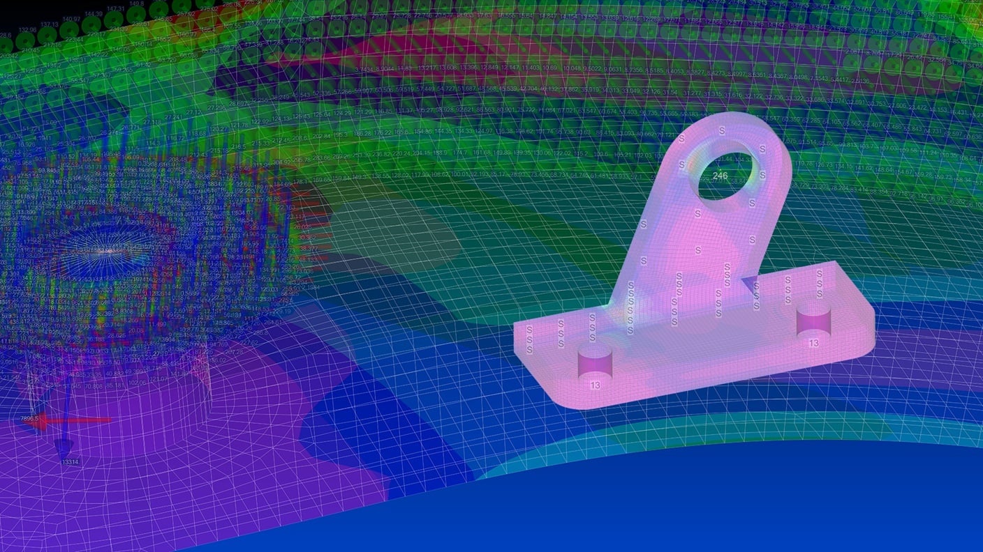
_{Here RBE “spider” elements (highlighted in yellow) are used for multiple purposes. (1) RBE3 to distribute bearing load at the lug. In this example the RBE3 dependent node DOF cannot not include DOFs 246 since these are included in the symmetry SPC (2) RBE2 used to model a bolted connection by connecting a beam element to a circular region (pad) of solid element nodes. This is also example of connecting elements with different DOFs using RBEs.}

Symmetry and Axisymmetry

Symmetry is one of the best ways to reduce model size—when it applies. If geometry, loading, and expected response are symmetric about one or more planes, symmetry constraints can be used.

On a symmetry plane, you typically constrain:

• • out-of-plane translation, and
  • in-plane rotations (for shell/beam formulations where those rotational DOFs exist)

Any loads intersected by the symmetry plane must be adjusted accordingly (for example, halving a point load if you model half the structure).

Multiple symmetry planes can reduce a model to 1/2, 1/4, 1/8, etc.

Axisymmetric analysis applies when geometry and loading can be revolved around an axis with no circumferential variation (common in pressure vessels and other bodies of revolution). This reduces the model dimension by one, creating very efficient models that still capture the full behavior:

• Thick-walled bodies: A thick-walled revolved solid body can be represented by a 2D r-z cross-section using axisymmetric solid elements. Although the mesh is 2D, the solution recovers the full axisymmetric 3D stress state (including hoop stress).
• Thin-walled bodies: A thin-walled revolved body can be represented with axisymmetric shell formulations, typically defined along a mid-surface (meridian) line in the r-z plane. Although the mesh is 1D, the solution captures the shell’s membrane and bending behavior for the full revolved geometry.

_{Here ½ symmetry was used to reduce the model size. Only sliding is allowed along the symmetry plane (yellow region). The applied load shown here would be ½ of the total loading because it is split by the plane of symmetry.}

Elastic Supports and Springs

Not all supports are rigid. You can represent support compliance in a few ways:

• • Model surrounding structure and constrain farther away (letting the model develop realistic flexibility).
  • Use spring elements to represent compliance directly.

Springs are also useful as stabilizers to prevent rigid-body motion with minimal load transfer (for example, very low stiffness in a direction you only need to restrain numerically).

Prescribed Displacement

Prescribed displacement is often more “load-like” than a traditional constraint: it enforces a displacement via constraint equations. It answers:

• • What stress/strain is required to achieve the displacement?
  • What reaction forces result?

This is especially useful for displacement-driven behaviors such as plastic snap fits, press fits, and interference assemblies.

Loads and Contact

Loads are often more intuitive than constraints, but they share a key similarity: even if you apply loads to faces or geometry in a preprocessor, the solver ultimately resolves them to nodal loads.

Common load types include:

• • Force / moment
  • Pressure
  • Enforced displacement / rotation
  • Bolt preload
  • Acceleration / velocity
  • Temperature

Use only loading that matches your question—and make sure the model supports it. For example:

• • acceleration loads require mass/density to produce forces
  • temperature changes require coefficient of thermal expansion (CTE) to produce thermal strain/stress

Contact can dramatically increase model complexity and make troubleshooting more difficult. If possible, get the model running without contact first, then add contact progressively.

If you only need one-way resistance (gap closure) in a localized area, consider simplified contact representations such as gap elements (where supported).

Keep in mind: contact that opens/closes or changes status is inherently nonlinear. Defining many contact pairs at once, especially in large models, can quickly make a model fragile and difficult to debug.

Model Checks and Side Studies

Poor boundary conditions often won’t prevent a model from running; even worse results may look reasonable at first glance. A few basic checks early can prevent a lot of wasted time.

• Check reactions: Do reaction forces and moments balance the applied loads? Are directions reasonable? Are there large opposing reactions that suggest over-constraint?
• Check deflections: Does the shape and magnitude match intuition?
• Interrogate hotspots: Are stress concentrations driven by real geometry/load paths—or by boundary-condition idealizations?

When models get complex, it can be hard to judge how much an assumption matters. One of the strengths of FEA is the ability to run controlled variants:

• Try a few spring stiffness values.
• Change how far away you place a “fixed” boundary in a compliance model.
• Compare RBE2 vs RBE3 behavior in a small test model.

Small side models that run in seconds are often the fastest way to build confidence in your idealizations before committing to a large model with many other assumptions layered in.

If your model is small enough you may be able to try different boundary condition configurations directly, otherwise, simplify with a coarse mesh first, try different boundary condition assumptions, and compare reaction forces to build intuition before refining and adding complexity.

An Example - Boundary Condition Idealization Comparison

In the following example, 4 models were compared using the same geometry and loading, but applying boundary conditions at the bolted interface in progressively more realistic ways. Comparing the reaction forces, deflections, and stress results between them illustrates how these choices affect what questions a model will be useful for answering.

• Model 1 – Bottom bolted surface fixed. This is a very poor modeling assumption but might be tempting for a new engineer.
• Model 2 – Bolt hole surfaces fixed.
• Model 3 – Bolt hole center points constrained in translation only, connected through RBE2 elements.
• Model 4 – Bolts modeled with beams, minimally constrained, connected through RBE2 elements.

Deflections and Stresses

_{Comparing multiple model variants — although each produces different deflections and reactions at the base plate, stress at the end of the lug is virtually identical across all four. Which model is acceptable depends on what question you are asking. Each model gets progressively more useful near the bolted interface, although none would be appropriate for extracting stresses at the bolted connections — that would require explicit fastener modeling with contact, which usually adds unnecessary complexity. Fastener loads are better obtained from the model and verified or analyzed with hand calculations.}

Reaction Forces

_{Model 1 had the entire bottom face fixed. Summing reaction forces at the bottom face verifies that the applied load is balanced. However, additional force and moment components are picked up that should be reacted by the symmetry plane, not the base. Individual bolt loads are also not readily available.}

_{Model 2 had translation in X, Y, and Z fixed at all bolt hole surface nodes. Summing reaction forces at bolt holes shows unexpected out of plane forces and large moments, suggesting an over-constrained model. Also note that center of reaction force is on midplane of plate.}

_{Model 3 had translation in Z and X fixed at a bolt reference node, which was connected to a circular washer pad on the mesh with RBE2 element. Reaction forces look better with only the expected components and no moments transferred through bolts. However, the large opposing forces in x suggest some over-constraint.}

_{Model 4 had bolts modeled with a beam and RBE2 elements. The RBE2 connects a washer pad on the top surface to beam at hole center. The beam then connects to a bolt reference node which had translation fixed in X and Z. This is the expected fastener load distribution, which should be very similar to hand calcs.}

Closing Thoughts

Good boundary conditions are less about checking the right boxes in your FEA software and more about preserving the physics of how forces enter and leave the structure. Constraints influence stiffness. Stiffness changes load paths. Load paths drive stress, deflection, fatigue life, and even contact behavior.

Treat boundary conditions as part of the design intent, not just model setup. Make the assumptions explicit, confirm equilibrium through reactions, and confirm behavior through deflection shape before you optimize geometry or debate hotspot values. That discipline is what separates an illustrative simulation from one you can confidently use to guide engineering decisions.

Need FEA support on your next project?  Get in touch.